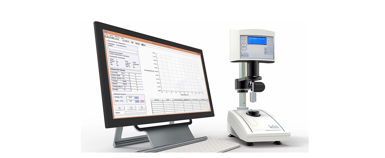
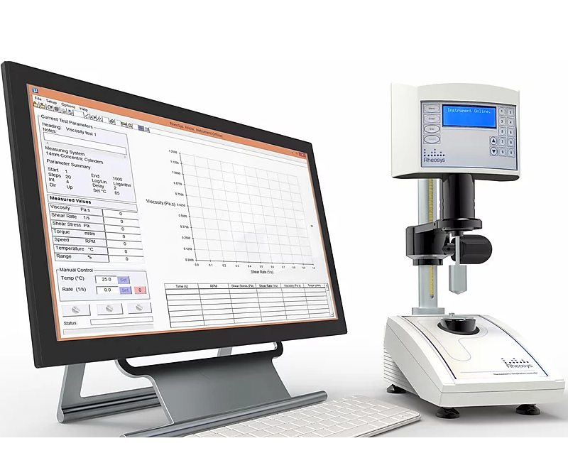
보유장비 (R&D Facility)
본 점도계는 -10℃ ~ 120℃ 의 온도범위에서 시료를 가열 냉각하여 온도의 함수로써 점도를 측정하는 스핀들 회전형 점도계입니다.
분석 문의하시면 2~3일 이내 데이터를 제공하고 측정 보고서 발행 가능합니다.
가압 조건의 점도 측정은 고주파 점도계로 서비스할 수 있습니다.
- 측정범위 : 1 cPs ~ 1,000,000 cPs
- 회전속도 : 0.1 ~ 2000 rpm
- Angular Velocity: 0.01 to 200 rad/s*
- Shear Rate: Measuring System Dependent
- Shear Stress: Measuring System Dependent
- 토크 범위 : 0 ~ 20 mNm
- Measuring Systems: Cone & Plate (CP), Parallel Plate (PP), Co-Axial Cylinders (CC), Vane Rotor
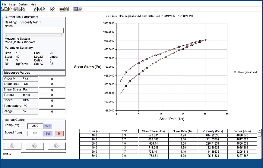
Data Displayed
Selected Speed (RPM / Sˉ¹)
Viscosity reading (cP / mPa.s)
Torque (mNm / %FS)
Sample Temperature (0.01 ºC)
Shear Rate (Sˉ¹)
Shear Stress (Pa. (N/m²))
Basic rheological terms
The following sections explain the basic terms such as stress and strain that are used in rheology & viscometry
Shear Strain.
To define the term STRAIN we will consider a cube of material with its base fixed to a surface as shown below in figure-1.
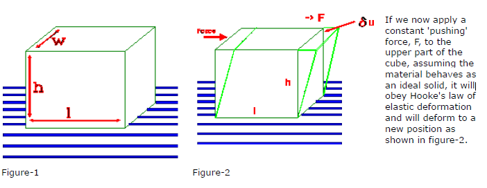
This type of deformation (lower fixed upper moving) is defined as a SHEAR DEFORMATION.
The deformation δ u and h are used to define the SHEAR STRAIN as :
Shear Strain = δ u/h
The shear strain is simply a ratio of two lengths (displacement / gap) and so has no units. It is important since it enables us to quote pre-defined deformations without having to specify sizes of sample etc.
Shear Stress.
The SHEAR STRESS is defined as F/A (A is the area of the upper surface of the cube l x w) Since the units of force are Newtons and the units of area are m2 it follows that the units of Shear Stress are N/M2 This is referred to as the PASCAL (i.e. 1 N/m2 = 1 Pascal) and is denoted by the symbol σ (in older textbooks you may see it denoted as τ)
Shear Rate.
Consider the case of a cube of material that behaves as an ideal fluid. When we apply a shear stress (force) the material will continually deform at a constant rate as illustrated in figure-4.
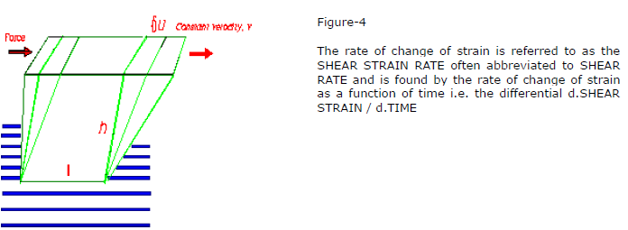
Typical Shear rate's for some standard processes
Process Typical range (S-1)
Spraying 104 to 105
Rubbing 104 to 105
Curtain coating 102 to 103
Mixing 101 to 103
Stirring 101 to 103
Brushing 101 to 102
Chewing 101 to 102
Pumping 100 to 103
Extruding 100 to 102
Levelling 10-1 to 10-2
Sagging 10-1 to 10-2
Sedimentation 10-1 to 10-3
Viscosity
The Shear Rate obtained from an applied Shear Stress will be dependant upon the materials resistance to flow i.e. its VISCOSITY
Since the flow resistance ≡ force / displacement it follows that ;
VISCOSITY = SHEAR STRESS / SHEAR RATE
The units of viscosity are Nm2s Which are better known as Pascal Seconds (Pa.s)
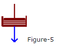
If a material has a viscosity which is independent of shear stress then it is referred to as an ideal or NEWTONIAN fluid.
The mechanical analogue of a Newtonian fluid is a viscous dashpot which moves at a constant rate when a load is applied as seen in figure-5.
Typical Viscosity Values
Material Approximate Viscosity (Pa.S)
Air 10-5
Acetone (C3H6O) 10-4
Water (H2O) 10-3
Olive Oil 10-1
Glycerol (C3H8O3) 10+0
Molten Polymers 10+3
Bitumen 10+8
Basic Viscometry Units:
Viscosity
1 Ns/m2 = 1 Pa.s = 10 Poise
Viscosity in Poise / Density = Kinematic viscosity in Stokes
Shear Stress
1 Pa = 1 N/m2 = 10 dyn cm-2
Torque
1 mNm = 9.81 gcm = 10000 dyne cm
Types of Viscometry test, Flow Characterization
The next section covers the definitions and explanation of basic flow characterization techniques.
The viscometry test
There are generally two types of simple flow characterization tests for viscometry . These are Stepped shear rate or Constant shear rate.
The types available on your particular instrument will depend upon the configuration of your rheometer software.
Stepped shear. Individual shear values are selected. Each shear is applied for a user set time and the shear rate, shear stress and viscosity are recorded for each value.
The individual points are then either joined up 'dot to dot' fashion or using a rheological model to produce the flow curve and the viscosity curve.
This test method is the generally the preferred way of generating flow and viscosity curves.
Types of flow curve
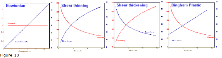
The measured viscosity of a fluid can often be seen to behave in one of four ways when sheared,
namely :
1. Viscosity remains constant no matter what the shear rate (Newtonian behavior)
2. Viscosity decreases as shear rate is increased (Shear thinning behavior)
3. Viscosity increases as shear rate is increased (Shear thickening behavior)
4. Viscosity appears to be infinite until a certain shear stress is achieved (Bingham plastic)
Over a sufficiently wide range of shears it is often found that the material has a more complex characteristic made up of several of the above flow patterns.
Flow curves
Since it is the relationship of shear stress to shear rate that are strictly related to flow we can directly show the flow characteristics of a material by plotting shear stress v shear rate. A graph of this type is called a Flow Curve. Figure-10 show the flow curves and viscosity curves of the four basic flow patterns.
The exact behavior of materials can often be described by some form of rheological model. Some of the more commonly used models are described in the following section.
Models for fundamental flow behavior
These models describe the simple flow behavior as shown in the previous graphs.
Most materials will start to deviate from these relationships over a sufficiently large shear range.
They are well suited to studying materials over a small shear range or where only a simple relationship is required.
Newtonian
This is the simplest type of flow where the materials viscosity is constant and independent of the shear rate. Newtonian liquids are so called because they follow the law of viscosity as defined by Sir Isaac Newton;
Shear Stress = Shear rate * viscosity
Water, oils and dilute polymer solutions are some examples of Newtonian materials.
Power law - (or Ostwald model)
Many non-Newtonian materials undergo a simple increase or decrease in viscosity as the shear rate is increased. If the viscosity decreases as the shear rate is increased the material is said to be "shear thinning" or "pseudo plastic". The opposite effect is known as shear thickening. Often this thickening is associated with a change in sample volume. This is called "dilatency".
The Power law is good for describing a materials flow under a small range of shear rates. Most materials will deviate from this simple relationship over a sufficiently wide shear rate range.
Shear stress = viscosity * Shear rate ^n
Where 'n' is often referred to the Power law index of the material.
If n is positive, material is shear thinning, if n is negative then material is shear thickening.
Polymer solutions and melts as well as some solvent based coatings show Power law behavior over limited shear rates.
Bingham
Some materials exhibit an 'infinite' viscosity until a sufficiently high stress as applied to initiate flow.
Above this stress the material then shows simple Newtonian flow. The Bingham model covers these materials;
Shear Stress = Limiting shear Stress + viscosity * shear rate
The limiting stress value is often referred to as the Bingham "yield stress" or simply the "yield stress" of the material. It should be noted that there are many definitions of Yield stress. For further information on this topic see the section on Yield values later.
Many concentrated suspensions and colloidal systems show Bingham behavior.
Herschel Bulkley
This model incorporates the elements of the three previous models
Shear stress = limiting stress + viscosity * shear rate^n
Special Cases of the model:
A pure Newtonian material has limiting stress=0 and n=0
A power law fluid has limiting stress=0 and n=power law index
A Bingham fluid has limiting stress= 'Yield value' and n=0
This models many 'industrial' fluids and so is often used in specifying conditions in the design of process plants.