Instruments to which this note applies: I-Cal Flex, Biocal
Prepared by: Lars Wadsö
Target use: organic decomposition, composting, aerobic biological activity
Introduction
퇴비화는 다른 종류의 유기물이 생물학적 활동에 의해 분해되는 중요한 과정입니다.이것은 토양에 추가하기 위한 적절한 형태로 된 혼합 유기물의 제어받은 호기성 개종으로서 정의할수 있습니다 [1]. 대부분의 경우 가장 활동적인 미생물은 박테리아와 곰팡이지만 벌레, 선충, 곤충과 같은 다른 유형의 동물도 그 역할을 할 수 있습니다. 퇴비는 소화조/발효조와 달리 호기성입니다.
퇴비화의 가장 일반적인 유형의 물질 중 하나는 목재, 톱밥 또는 빨대와 같은 리그 노셀룰로오스 재료입니다. 이러한 물질은 일반적으로 탄소가 높고 질소가 적으며 주로 곰팡이에 의해 분해됩니다. 잘려진 잔디, 잡초, 나뭇잎 그리고 나뭇가지와 같이 잘려진 나무로 된 정원 퇴비와 같은 혼합 퇴비에서 후자는 낮은 C/N 값인 500을 가지고 다른 물질에 비해 크기도 큽니다. 나무조각이 많은 퇴비는 성숙하기까지 몇 년이 걸립니다.
이 응용자료는 퇴비에서 목재 재료의 분해 속도를 평가하기 위해 등온 열량 측정법을 사용하는 방법을 설명합니다.
Materials and methods
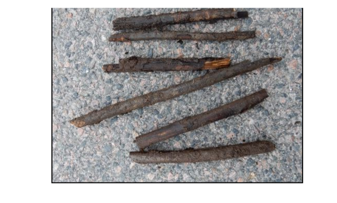
Wood twigs with diameters of 10-15 mm (Fig. 1) were taken out of a garden compost, cut into 40 mm lengths, and inserted in 20 mL polymer vials for calorimetric measurements in an I-Cal Flex calorimeter. The tests were conducted at two temperatures: 12 and 27 °C.
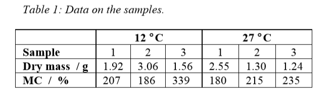
Three 40 mm twigs were measured at the two abovementioned temperatures. The masses and dry base moisture contents (MC) are detailed in Table 1.
garden compost
The samples were loaded into the calorimeters without any pre-thermostating. The calorimeters had been electrically calibrated and 4 mm stainless steel disks were used as references.
Results and discussion
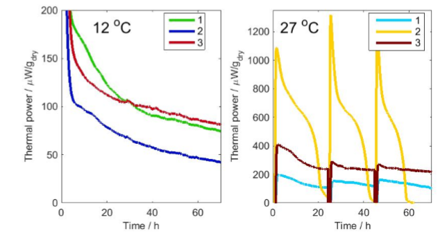
Figure 2 shows the results of the measurements. Note that the thermal powers were normalized per gram dry sample. The thermal power – and thus the rates of degradation are lesser at the lower temperature, as can be expected. There are also some differences between the various samples. For example, sample 2 at 27 °C has significantly higher thermal powers than the other samples, and runs out of oxygen after about 20 hours of degradation (see discussion below). As the measurements were made in closed vials, the result was affected by the changing gas composition in the vials, and therefore the samples at the higher temperature were aerated twice (after 20 hours and 40 hours), which corresponds to the times when the activity of sample 2 had gone down to close to zero.
The main degraders of wood are fungi, and we can assume that most of the heat measured comes from aerobic fungal respiration. As respiration produces 455 kJ of heat per mol oxygen consumed [2], the results in Fig. 2 can be recalculated to oxygen consumption rates. This has two immediate uses in this case: understanding the effect of changes in gas composition in the closed vials, and calculating the rate of wood degradation.
During a respiration measurement in a closed vial, the oxygen concentration decreases and the carbon dioxide concentration increases. In most cases it is the increase in carbon dioxide that will influence the activity most. In this experiment the vials have a volume of about 21 mL.
Let’s take a closer look at sample 2. This sample occupied about 4 mL of vial space, leaving about 17 mL of air (with 21% oxygen) at the start of the measurements. Using the ideal gas law, we can calculate that the quantity of O2 in moles present at the onset of the experiment.
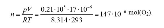
We used a temperature of 20 °C as a mean temperature of the two measurements. If we multiply this amount of oxygen by the enthalpy 455 kJ/mol(O2), we get 67 J. We can thus get a maximum of 67 J from the respiration of the sample with the amount of oxygen present in the head-space of the vial. To validate this, we have plotted in Fig. 3 the heat produced as a function of time for sample 2 at 27 °C. The graph shows that the heat actually peaks at about 50 J, a value 25% lower than 67 J. Possible reasons for this are that more oxygen is consumed during the first hour than is measured because of the initial disturbance in the calorimeter signal, or that the activity goes to lower levels as a result of the combined effect of decreasing oxygen and increasing carbon dioxide concentrations. In any case, we can infer that the decrease in the signal seen in the results is an effect of the change in gas composition in the closed vials. Another interesting point is that sample 2 at 27 °C immediately recovers its activity after aeration, which suggests that it is not harmed or inhibited by the changes in gas concentrations. Also note the decreasing amplitude of the successive peaks in Fig. 3 gets lower, which may be because the aerations were too short and therefore did not completely refresh the atmosphere in the vials.
Now let’s calculate the rate of degradation. If we assume that carbohydrate is what is consumed, the overall reaction is (with CH2O being a carbohydrate repeating unit):
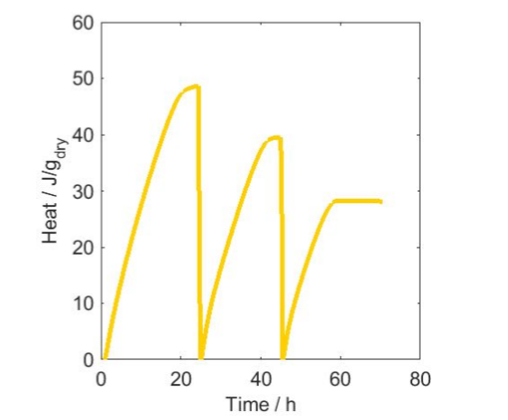
has been set to zero at each aeration
and since we know the oxygen consumption rate we can calculate the carbohydrate degradation rate. Taking sample 2 at 12 °C as an example, and using the initial 100 µW thermal power per gram dry mass, this can be recalculated to about 0.2 nmol/s carbohydrate consumed (using the 455 kJ/mol(O2) enthalpy).
As the molar mass of the carbohydrate repeat unit is 30 g/mol, this value corresponds to 6 ng degradation per s per g of material, or about 1.5% degradation per month.
The simple calculations above highlight some of the uses of isothermal calorimetry as an interesting technique to study biological processes such as composting.
References
- Hubbe, M.A., M. Nazhad, and C. Sánchez, Composting as a way to convert cellulosic biomass and organic waste into high-value soil amendments: A review. BioResources, 2010 5(4) 2808-2854.
- Criddle, R.S., A.J. Fontana, D.R. Rank, D. Paige, L.D. Hansen, and R.W. Breidenbach, Simultaneous measurement of metabolic heat rate, CO2 production and O2 consumption by microcalorimetry. Anal. Biochem., 1991 194 413-417.
- Formula of the quantity of O2.png (10.53kB)
- Table 1 - Data on the sample.png (25.54kB)
- Fig. 2 – The results of the measurements at two temperatures..png (128.38kB)
- Fig. 1 – Wood twigs with diameters of 10-15 mm taken from a garden compost.png (321.12kB)
- Formula of Formaldehyde and oxygen.png (4.11kB)
- Fig. 3 – The heat produced by sample 2 at 27 ° C. The heat has been set to zero at each aeration.png (71.33kB)
